Understanding Self-Attention from First Principles

Sun Jun 07 2026

Self-Attention from First Principles. I have read a lot of articles and watched many videos, and I noticed that no one explains this incredibly important topic in the easiest manner.

$$\text{Attention}(Q, K, V) = \text{softmax}\left(\frac{QK^T}{\sqrt{d_k}}\right)V$$

Most resources require you to be highly proficient in Deep Learning and its advanced mathematics to fully grasp the concepts.

But Self-Attention is actually simple if learned the right way.

At its core, Self-Attention relies on just three foundational components:

Dot Product (The Matching Tool)
Weights (The Learnable Transformation)
Data (The Values to Transmit)

Self-attention was the core innovation that enabled the Transformer architecture, which ultimately transformed modern AI, that we see today.

I won't start with abstract formulas, instead,

I will break things down in the simplest way possible by giving you raw intuition first, building up to the complete mathematical matrix.

Let's begin.

Step 1: We Have a Sentence

"My name is Ankit"

The Tokenizer converts these words into numerical IDs:

[523, 1024, 98, 4567]

These numbers are just IDs with no inherent meaning yet. Think of them as simple mappings:

My     = 523
name   = 1024
is     = 98
Ankit  = 4567

They are just labels, exactly like a Student ID or an Employee ID.

Step 2: Embedding Layer

Now we need to add meaning. Suppose our embedding dimension is 2 for learning purposes. The model uses a large lookup table called an embedding table:

Token ID	Embedding Vector
523	$[0.12, \phantom{-}0.33]$
1024	$[0.51, -0.20]$
98	$[0.22, \phantom{-}0.78]$
4567	$[0.88, \phantom{-}0.12]$

Mapping our tokens to vectors gives us this structured representation:

Word	Dimension 1	Dimension 2	Vector Representation ($\vec{x}$)
My	0.12	0.33	`[0.12, 0.33]`
name	0.51	-0.20	`[0.51, -0.20]`
is	0.22	0.78	`[0.22, 0.78]`
Ankit	0.88	0.12	`[0.88, 0.12]`

Question: What does a vector like `[0.12, 0.33]` actually mean?

Answer: Nobody knows exactly. This is a very important concept to understand.

People often assume:

0.12 = person score
0.33 = noun score

This is not true. The vector represents a compressed meaning.

Step 3: Put All Embeddings Together

Next, we stack these individual vectors together into a single data matrix, which we call $X$. Let's break down the assembly of this matrix line by line, mapping each word to its specific row.

First, we take the vector for My:

X =

[
  [0.12, 0.33]
]

Next, we stack the vector for name directly underneath:

X =

[
  [0.12, 0.33],
  [0.51, -0.20]
]

Then, we append the vector for is:

X =

[
  [0.12, 0.33],
  [0.51, -0.20],
  [0.22, 0.78]
]

Finally, we add the vector for Ankit to complete our sequence:

X =

[
  [0.12, 0.33],
  [0.51, -0.20],
  [0.22, 0.78],
  [0.88, 0.12]
]

To visualize this explicitly, we can view the finished matrix with its corresponding word rows:

X =

[
  [My],
  [name],
  [is],
  [Ankit]
]

[
  [0.12, 0.33],
  [0.51, -0.20],
  [0.22, 0.78],
  [0.88, 0.12]
]

Shape of X

Rows = 4: Because we have 4 tokens (My, name, is, Ankit).
Columns = 2: Because our embedding dimension is 2.

Therefore, the shape of our matrix is:

$$X \in \mathbb{R}^{4 \times 2}$$

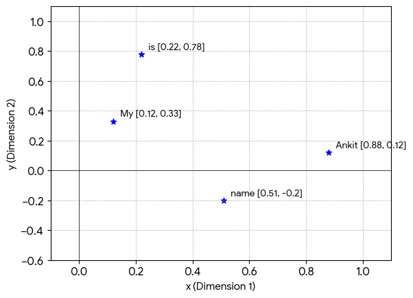
Visualization

Think of each word as a point in an embedding space.

The coordinates of the point are the values inside the embedding vector.

For example:

My → [0.12, 0.33] name → [0.51, -0.20] is → [0.22, 0.78] Ankit → [0.88, 0.12]

In this toy 2D example, each embedding can be visualized as a point on a graph.

An Important Realization

At this stage:

My does NOT know that name exists.
Ankit does NOT know that My exists.

Each token is completely independent. We only have Word Meaning, not Sentence Meaning yet.

What Problem Does Attention Solve?

Currently, we know:

Ankit = [0.88, 0.12]

But the vector for Ankit has no idea it is appearing inside the specific sentence "My name is Ankit".

The model needs Ankit to learn that it is contextualized by and related to My, name, and is.

This is the exact motivation for Self-Attention.

Before Q, K, V: Raw Intuition

Let's ask a fundamental question:

If I am the word "Ankit", how can I determine which other words in this sentence are important to me?

A simple, intuitive approach is to compare my embedding with every other embedding using a mathematical operation called the dot product:

Ankit $\leftrightarrow$ My
Ankit $\leftrightarrow$ name
Ankit $\leftrightarrow$ is

This gives us our very first attention intuition: measuring similarity between words.

The Math: Computing Dot Products Manually

Let's compute the similarity scores for the word Ankit on paper.

Our Embeddings Reference

My: [0.12, 0.33]
name: [0.51, -0.20]
is: [0.22, 0.78]
Ankit: [0.88, 0.12]

What is a Dot Product?

For two vectors $\vec{a} = [a_1, a_2]$ and $\vec{b} = [b_1, b_2]$, the dot product is calculated by multiplying corresponding elements and summing them up:

$$\vec{a} \cdot \vec{b} = a_1b_1 + a_2b_2$$

Dot Product 1: Ankit $\cdot$ My

$$[0.88, 0.12] \cdot [0.12, 0.33]$$

Step 1: $0.88 \times 0.12 = 0.1056$
Step 2: $0.12 \times 0.33 = 0.0396$
Step 3: $0.1056 + 0.0396 = 0.1452$

$$\text{Ankit} \cdot \text{My} = 0.1452$$

Dot Product 2: Ankit $\cdot$ name

$$[0.88, 0.12] \cdot [0.51, -0.20]$$

Step 1: $0.88 \times 0.51 = 0.4488$
Step 2: $0.12 \times (-0.20) = -0.0240$
Step 3: $0.4488 - 0.0240 = 0.4248$

$$\text{Ankit} \cdot \text{name} = 0.4248$$

Dot Product 3: Ankit $\cdot$ is

$$[0.88, 0.12] \cdot [0.22, 0.78]$$

Step 1: $0.88 \times 0.22 = 0.1936$
Step 2: $0.12 \times 0.78 = 0.0936$
Step 3: $0.1936 + 0.0936 = 0.2872$

$$\text{Ankit} \cdot \text{is} = 0.2872$$

Dot Product 4: Ankit $\cdot$ Ankit

$$[0.88, 0.12] \cdot [0.88, 0.12]$$

Step 1: $0.88 \times 0.88 = 0.7744$
Step 2: $0.12 \times 0.12 = 0.0144$
Step 3: $0.7744 + 0.0144 = 0.7888$

$$\text{Ankit} \cdot \text{Ankit} = 0.7888$$

Final Similarity Scores For "Ankit"

Compared With	Dot Product Score
Ankit	0.7888
name	0.4248
is	0.2872
My	0.1452

In this toy embedding space, Ankit is mathematically closest to itself, followed by name, is, and lastly My.

Why Does the Dot Product Measure Similarity?

Aligned Vectors: If two vectors point in a highly similar direction, their dot product yields a large positive value.
Opposite Vectors: If two vectors point in completely opposite directions, their dot product yields a negative value.
Orthogonal Vectors: If two vectors point at a $90^\circ$ angle to each other, their dot product is exactly $0$ (completely unrelated).

Large Positive Score $\rightarrow$ Similar direction

Near Zero Score $\rightarrow$ Unrelated

Negative Score $\rightarrow$ Opposite direction

Why Simple Dot Products Are Limiting

If we calculate attention scores directly using our raw input embeddings, we are effectively doing a pure matrix multiplication:

$$\text{Score} = XX^T$$

This is a fixed geometric calculation. Because there are no additional learnable parameters involved in deciding how tokens should interact, the model can only rely on whatever static features already exist inside the pre-trained embeddings.

As a result, the model is strictly limited to measuring the similarity of dictionary meanings, rather than the relevance of situational relationships.

The "Apple Watch" Problem

Consider how a model handles this sentence using raw embedding dot products:

"I love Apple Watch"

The model looks at Apple and Watch as completely separate items. It computes the dot product of their static embeddings ($Embedding_{\text{Apple}} \cdot Embedding_{\text{Watch}}$) to find their similarity:

Apple in a dictionary space sits close to fruits like Banana or Orange.
Watch in a dictionary space sits close to verbs like Look or See, or instruments like Clock.

Because their dictionary meanings are completely different, their raw dot product score is incredibly low. The model completely misses the fact that when these two words sit next to each other, they instantly bind together to form a single luxury tech product.

Visualizing the Bottleneck

If we plot this on a 2D graph, you can instantly see why raw embeddings fail to capture the true context of the sentence:

  Dim 2 ▲
        │          [Clock]
        │             ▲
        │             │  (Far apart! Low dot product)
        │             ▼
        │          [Watch] ───► [Look/See]
        │
        │
        │  [Apple] ───► [Banana/Orange]
        │
────────┴──────────────────────────────────► Dim 1

Looking at the graph, Apple and Watch are trapped in completely different neighborhoods. A simple dot product cannot bridge this gap because it doesn't have any moving parts to learn why they should interact.

What We Actually Need the Model to Learn

Language isn't a static dictionary. The meaning of a word changes dynamically based on its neighbors:

Apple + Watch  ➔  Smartwatch Product (Technology)
Apple + Pie    ➔  Baked Dessert (Food)
Watch + Movie  ➔  Action Verb (Entertainment)

To give the AI this context-shifting superpower, we need a system that can stretch, rotate, and transform our original embedding space depending on the task at hand.

This is exactly why Transformers introduce three specialized, trainable weight matrices: $W_Q$ (Query), $W_K$ (Key), and $W_V$ (Value). These parameters act like custom, adjustable lenses that transform words from a space optimized for static meaning into a new space optimized for dynamic relationships.

The Self-Attention Formula: Breaking Down the Pieces

Before we watch the matrices clash, let's look at the actual mathematical formula that ties everything together:

$$\text{Attention}(Q, K, V) = \text{softmax}\left(\frac{QK^T}{\sqrt{d_k}}\right)V$$

Let's break down exactly what each piece of this formula is doing before we calculate it:

$QK^T$ (The Matching Engine): This is the row-by-row dot product multiplication. It is where every Query asks every Key: "How relevant are you to me?"
$\sqrt{d_k}$ (The Scaler): This is a safety buffer. $d_k$ is the dimension size of our keys. If our dimensions get too large, the dot product scores blast through the roof, which breaks the math during training. Dividing by $\sqrt{d_k}$ keeps the numbers stable.
$\text{softmax}(\dots)$ (The Normalizer): This is the activation function that turns our raw matching scores into probabilities (ranging from 0 to 1).
$V$ (The Information Carrier): Finally, we multiply those percentages by the actual data payload matrix ($V$) to extract the exact contextual meaning we need.

Now, let's look at the raw matrix mechanics of just that first crucial step: the matching engine, $QK^T$.

Enter Q, K, and V

Instead of forcing a single embedding vector to do everything, Transformers introduce three separate, trainable weight matrices: $W_Q$ (Query Weight), $W_K$ (Key Weight), and $W_V$ (Value Weight).

These matrices are initialized with random numbers and optimize themselves over time using backpropagation. By multiplying our raw input matrix $X$ with these weights, we generate three entirely distinct operational spaces:

$$Q = X \cdot W_Q \quad \text{(Queries)}$$

$$K = X \cdot W_K \quad \text{(Keys)}$$

$$V = X \cdot W_V \quad \text{(Values)}$$

Query ($Q$): "What am I looking for?" (e.g., Ankit is looking for an introductory context word)
Key ($K$): "What characteristics do I possess?" (e.g., name says "I am an introduction placeholder tag")
Value ($V$): "What actual information do I carry?" (The actual content passed forward)

With Q and K ($Q_i \cdot K_j$)

Asks contextual relationship questions:

"How much should token $i$ pay attention to token $j$ right now given their roles in this sentence?"

The Math of $QK^T$: Step-by-Step Matrix Mechanics

Let's watch the magic happen mathematically. Let's look exclusively at the matrix multiplication $Q K^T$. We will forget Softmax and $V$ for a brief moment just to master how queries match keys.

Assume our text matrix has been projected into $Q$ and $K$ spaces (using 2-dimensional representations for simplicity):

Q (Query Matrix)

[
  [1, 0], // My Query
  [0, 1], // name Query
  [1, 1], // is Query
  [2, 1]  // Ankit Query
]

K (Key Matrix)

[
  [1, 1], // My Key
  [0, 2], // name Key
  [1, 0], // is Key
  [2, 1]  // Ankit Key
]

Both matrices have a shape of $(4, 2)$ because we have $4 \text{ tokens} \times 2 \text{ dimensions}$.

To perform a dot product of every row in $Q$ with every row in $K$, we transpose $K$ so it has a shape of $(2, 4)$:

Kᵀ (Key Matrix Transposed)

[
  [1, 0, 1, 2],
  [1, 2, 0, 1]
]

Now we compute the matrix multiplication: $Q_{(4 \times 2)} \times K^T_{(2 \times 4)} = \text{Score}_{(4 \times 4)}$. Why $4 \times 4$? Because every single token compares itself with every single token!

Computing Row 1: The "My" Token Perspective

We take the Query vector for My ($[1,0]$) and cross-multiply it with all word Keys in $K^T$:

My Query $\cdot$ My Key: $[1,0] \cdot [1,1] = 1(1) + 0(1) = \mathbf{1}$
My Query $\cdot$ name Key: $[1,0] \cdot [0,2] = 1(0) + 0(2) = \mathbf{0}$
My Query $\cdot$ is Key: $[1,0] \cdot [1,0] = 1(1) + 0(0) = \mathbf{1}$
My Query $\cdot$ Ankit Key: $[1,0] \cdot [2,1] = 1(2) + 0(1) = \mathbf{2}$

Row 1 results in: [1, 0, 1, 2]

Computing Row 4: The "Ankit" Token Perspective

We take the Query vector for Ankit ($[2,1]$) and cross-multiply it with all word Keys in $K^T$:

Ankit Query $\cdot$ My Key: $[2,1] \cdot [1,1] = 2(1) + 1(1) = \mathbf{3}$
Ankit Query $\cdot$ name Key: $[2,1] \cdot [0,2] = 2(0) + 1(2) = \mathbf{2}$
Ankit Query $\cdot$ is Key: $[2,1] \cdot [1,0] = 2(1) + 1(0) = \mathbf{2}$
Ankit Query $\cdot$ Ankit Key: $[2,1] \cdot [2,1] = 2(2) + 1(1) = \mathbf{5}$

Row 4 results in: [3, 2, 2, 5]

The Complete $QK^T$ Score Matrix

Filling out the entire matrix gives us an actionable relationship grid:

QKᵀ (Attention Score Matrix)

[
  [           My (K), name (K), is (K), Ankit (K) ],
  [ My (Q),        1,        0,      1,         2 ],
  [ name (Q),      .,        .,      .,         . ],
  [ is (Q),        .,        .,      .,         . ],
  [ Ankit (Q),     3,        2,      2,         5 ]
]

💡 The Deep Reading Intuition: Always read this matrix row by row. The row belongs to the Query (the word asking the question), and the columns belong to the Keys (the tokens responding). Looking at the Ankit row, its scores are [3, 2, 2, 5]. This means that while processing the word Ankit, the model determines it is highly self-relevant ($5$), but its strongest structural connection out of the remaining tokens is to the word My ($3$).

What Happens Next: Softmax and the Value Matrix ($V$)

Once we have our score matrix, we finish the rest of the standard attention pipeline:

1. Scaling and Softmax

We turn these raw score matrices into percentages. For example, applying Softmax to the Ankit row [3, 2, 2, 5] converts those numbers into normalized probabilities that equal $100%$:

Ankit Attention Weights: [ My: 12%,  name: 5%,  is: 5%,  Ankit: 78% ]

2. Gathering the Values ($V$)

Now that we know exactly how much attention to pay to each word, we multiply these percentage weights by the Value Matrix ($V$).

Instead of passing the original data or keys forward, we pull information directly from $V$. If a token has an attention score of $78%$ on itself and $12%$ on My, its final output vector will be a blended compound containing $78%$ of its own value profile and $12%$ of My's value profile.

Comment down your thoughts below, if you found it helpful !

here is the Research Paper : "Attention Is All You Need"-https://arxiv.org/pdf/1706.03762

Best,
Ankit

← Back to Blog ← Back to Home